Learning Oxford Nanopore's Basecalling Algorithms
Introduction
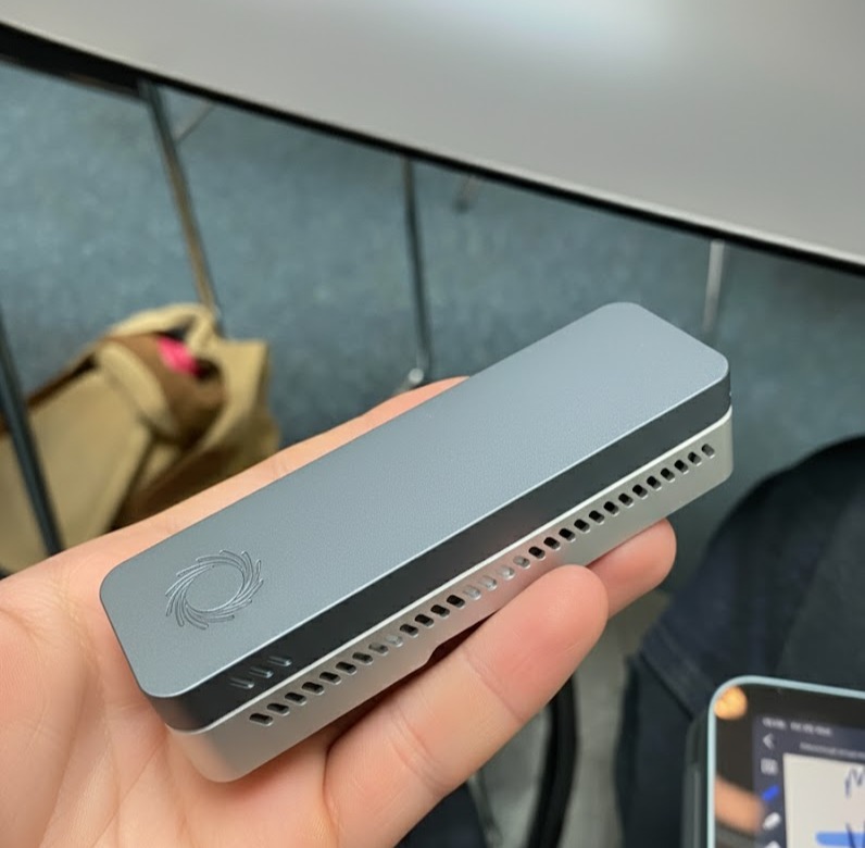 Oxford Nanopore's MinION.
After seeing and holding Oxford Nanopore's MinION during a talk at Imperial College London, I was impressed at the portability of the device, and I wondered how such a small device could so conveniently produce so much raw sequencing data. I was particularly interested at how the electrical currents flowing through nanopores could suddenly be interpreted as combinations of the bases and converted into DNA sequences. This process, called basecalling, sits at the heart of nanopore sequencing technology, and I decided to try and understand the algorithms behind it beyond simply reading papers. This included building my own tools and coding practical implementations to explore how basecalling works from the ground up.
This blog post documents my learning journey – the code I wrote, the challenges I faced, the insights I gained, and the deeper appreciation I developed for the computational complexity behind what appears to be a simple biological process. Whether you're a student, a bioinformatics researcher, or just curious about how cutting-edge genomics technology works, I hope this exploration provides valuable insights.
Background: What is Basecalling and Why Does It Matter?
Nanopore sequencing works by monitoring electrical current as DNA molecules pass through biological or synthetic pores. Each of the four DNA bases (A, T, G, C) creates a characteristic disruption in the current, producing a unique electrical "signature." The challenge lies in converting these noisy, complex electrical signals into accurate DNA sequences – this is basecalling.
The importance of basecalling cannot be overstated. Unlike traditional sequencing methods that produce sequences hours or days after sample preparation, Oxford Nanopore's technology enables real-time basecalling, allowing researchers to make decisions about their experiments while sequencing is still ongoing. This capability has revolutionized applications from outbreak monitoring to personalized medicine.
However, the computational challenge is immense. The basecaller must process thousands of electrical measurements per second, distinguish signal from noise, handle variable translocation speeds, and maintain high accuracy – all while keeping pace with the data generation rate of modern nanopore devices.
Understanding the Data Pipeline
The first step in learning about basecalling was getting familiar with nanopore data formats and understanding what the raw signals actually look like. I started by working with publicly available datasets from Oxford Nanopore's AWS repository, focusing on the POD5 file format that has replaced the older FAST5 format.
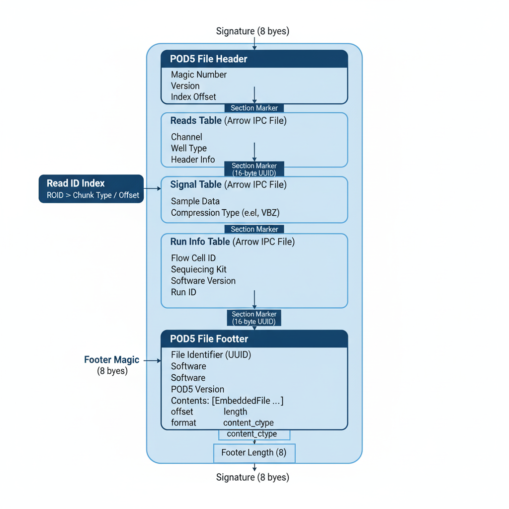 POD5 File Architecture.
The POD5 file format is a robust container designed to efficiently store nanopore sequencing data. At its core, it bundles multiple high-performance Apache Arrow tables, including the Reads table for metadata, the Signal table for raw electrical data, and the Run Info table for experimental details. The entire file is framed by a unique signature at both the beginning and end to verify its integrity. A crucial feature is the footer located at the very end of the file, which acts as a table of contents, detailing the exact location and size of each embedded data table. This design allows the sequential adding of data, which is essential for live sequencing runs.
Despite the sophisticated structure, accessing POD5 data was relatively simple, using a pod5.Reader object within a with statement. This reader object is itself an iterator, so you can use it directly in a simple for loop. On each pass of the loop, you are given a complete ReadData object containing all the data and metadata for a single read, allowing me to process each read sequentially with ease. Here’s how my main_test.py script uses the loader to get the specific read needed for the pipeline:
from pod5_data_loader import Pod5DataLoader

# The path to my specific data file and the target read
file_path = r"data\raw_pod5\HG002_raw_read.pod5"
read_id = "2536858a-ed8f-4e09-8dfe-15d7e2dd57c9"

# My custom class makes loading the data clean and safe
with Pod5DataLoader(file_path) as loader:
    # The method handles finding the specific read and extracting its signal
    signal_data = loader.load_signal_data(read_id=read_id)
    raw_signal = signal_data[0]['raw_signal']

print(f"Successfully loaded read {read_id} with {len(raw_signal)} data points.")
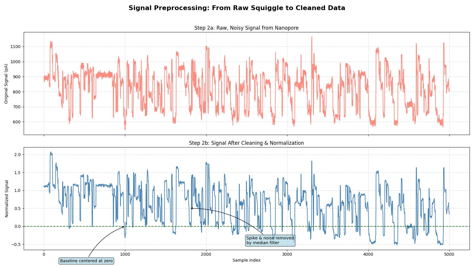
The raw data revealed the complexity immediately apparent in basecalling. Unlike the clean, discrete peaks you might expect, nanopore signals are continuous, noisy, and overlapping. Each "event" in the signal corresponds not to a single base, but to a k-mer (typically 5-6 bases) sitting in the pore simultaneously.
With this robust loader, I have a reliable and standardized way to get any raw signal data I need for the rest of the project. But this signal is still raw and messy. Before we can align it or train a model, it needs a serious clean-up.
To tame this noise, I developed a SignalPreprocessor pipeline that systematically cleans the data. It first clips extreme artifacts, then applies a median filter to eliminate sharp spikes without blurring the important event boundaries. Next, it flattens the signal by fitting and subtracting a polynomial to correct for baseline drift, and finally, it normalizes the entire stream using a RobustScaler to make the data stable and cantered around zero, resistant to any remaining outliers. The result is a transformation from a chaotic electrical scribble into a clean, analysable signal where the distinct levels corresponding to k-mers are finally visible.
 POD5 File Architecture.
The next aim was finding the raw signal's origin within its original genome—a true needle-in-a-haystack problem. For this, the SignalAligner class is designed to pinpoint the signal's genomic home. It hinges on a powerful algorithm called Dynamic Time Warping (DTW). The process is conceptually simple: I slide a window across the reference genome, convert the DNA sequence within that window into a theoretical "ideal" signal using a k-mer model, and then use DTW to measure how well my real, preprocessed signal matches this ideal one. DTW is brilliant here because it can find the best alignment even if the DNA didn't move through the pore at a perfectly constant speed. This process is repeated for thousands of overlapping windows, with each alignment producing a "distance" score—the lower the score, the better the match. Of course, searching millions of bases this way would be incredibly slow, so I implemented a crucial two-pronged optimization. First, the initial search uses downsampled, lower-resolution signals for a rapid comparison. Second, and most importantly, the entire search is massively parallelized using Python's multiprocessing module, distributing the work of checking hundreds of windows simultaneously across all available CPU cores. This parallel aligner chews through the vast search space, ultimately pinpointing the single genomic window with the lowest DTW distance, giving us the closest "ground truth" sequence corresponding to our read.
Now, with the aligned and pre-processed raw signal, the data is ready for basecalling.
Basecalling Architecture Deep-Dive
Basecalling algorithms have evolved significantly in the last ten years. Early basecallers relied on Hidden Markov Models (HMMs), which provided a statistical framework for modelling the relationship between electrical current signals and the underlying DNA sequence. These models typically used state emission densities, and leveraged algorithms like the modified Baum-Welch and Viterbi for training and inference. HMM's had issues in accurately identifying homopolymer regions where signals from identical sequential bases tend to merge, causing a significant number of deletion errors, requiring a different, more effective approach moving forward.
The breakthrough came with neural networks.
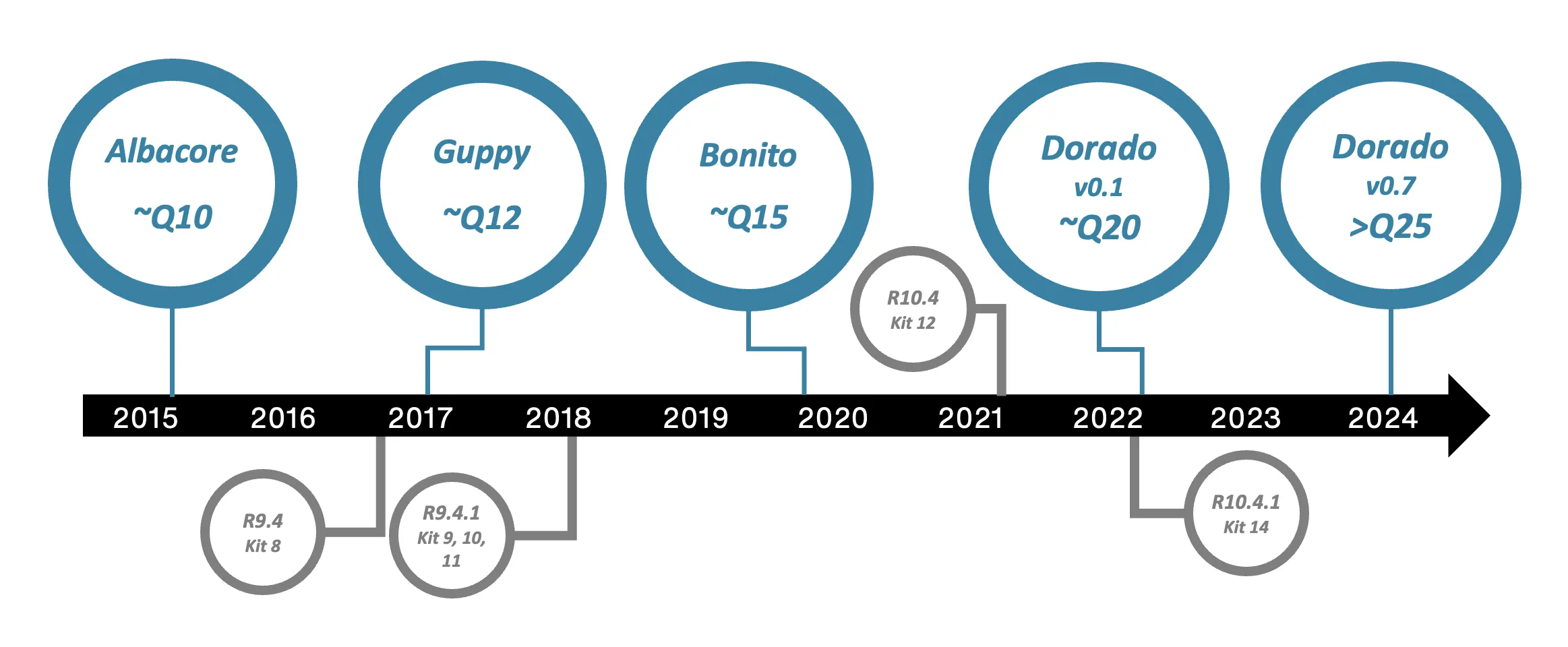
Albacore marked Oxford Nanopore’s transition away from HMMs toward neural network-based basecalling. It was the first to perform "raw basecalling," directly transforming electrical signals into DNA sequences without relying on an intermediary ‘event detection’ stage. Recurrent neural networks (RNNs) were used in Albacore to notably improve consensus accuracy and resolve longer homopolymers. This brought substantial gains in both single-read and overall sequence accuracy.
Guppy basecaller used RNNs with Connectionist Temporal Classification (CTC). CTC allowed the network to effectively handle the variable-length alignment problem inherent in nanopore data, mapping long raw signal sequences to shorter base sequences. Guppy delivered higher accuracy and throughput, quickly becoming the standard production basecaller due to its robustness and speed.
Bonito served as a research-focused, open-source basecaller, exploring hybrid architectures. Its model combined convolutional layers (for local signal feature extraction and noise reduction) with long short-term memory (LSTM) layers, which maintain context across long stretches of sequential data. Bonito further improved decoding by introducing a conditional random field (CRF) output head, enabling more nuanced alignment between signal features and base sequences. Bonito played an important role in driving new innovation, though mainly used for model development and benchmarking.
Dorado represents the latest leap, moving to advanced transformer architectures. Transformers, known for their self-attention mechanism and high parallelism, allow the model to consider long-range dependencies within the signal and extract richer information from the raw data. Dorado’s transformer-based design achieves both significantly higher accuracy and faster processing speeds, and it is optimized for high-throughput basecalling. It can also detect modified bases and supports duplex basecalling for epigenetic analyses.
Building My Own HMM
Basecalling using an HMM is like a detective story: we have the "observations" (the clues, which are our electrical signal points), and we want to infer the sequence of "hidden states" (the unseen events, which are the DNA k-mers that produced the signal). My entire hmm_basecaller.py script is dedicated to building, training, and using this model.
The model has three key components it needs to learn:
Emission Probabilities:
If the DNA k-mer 'ATCGT' is in the pore (a hidden state), what is the probability of observing a signal value of 95.3 pA (an observation)? I modelled this as a simple bell curve (a Gaussian distribution) for each of the 1024 possible 5-mers.
Transition Probabilities:
If the current k-mer is 'ATCGT', what is the probability that the next one will be 'TCGTT'? Or, what is the probability that the DNA pauses and the state remains 'ATCGT' for the next few signal points?
Initial Probabilities:
What is the probability that the read starts with any given k-mer?
To teach my HMM these rules, I implemented a two-phase training regimen.
Phase 1: Supervised Training
First, I used the aligned signal and reference sequence for a round of supervised training. In the train_supervised method, I grouped all the signal segments that corresponded to a known k-mer. For every single k-mer (like 'AAAAA', 'AAAAC', etc.), I calculated the the mean and standard deviation of the signal. This directly taught the HMM the initial emission probabilities—it now had a solid, data-driven starting point for what signal to expect for each k-mer.
Phase 2: Unsupervised Refinement
The initial training is good, but it's based on a slightly imperfect alignment. To create a truly robust model, I implemented the Baum-Welch algorithm in my baum_welch_train method. This is an unsupervised learning step that iteratively refines all the HMM's parameters—emissions, transitions, and initial probabilities—to find the set of values that best explains the entire observed signal. It's a process where the model essentially fine-tunes itself, learning the nuances of DNA translocation speed, like the precise probability of the DNA pausing versus moving forward.
This iterative process is computationally brutal. Running these algorithms in pure Python would take ages. To solve this, I used Numba, a just-in-time compiler. By adding a simple @njit decorator to my core HMM functions, Numba translates the slow Python loops into fast machine code, providing a speedup of over 100x and making the training process feasible.
The Final Basecalled Sequence
Finally, I implemented the Viterbi algorithm within my hmm_basecaller.py script. While the Baum-Welch training considered the probability of all possible paths to learn the model's rules, Viterbi's job is to find the single most probable path through those hidden states. It marches along the entire electrical signal, and at every single time point, it makes the optimal decision, asking: "Given the signal I see now and the rules I've learned, what is the most likely k-mer to be in this pore?" This dynamic programming approach efficiently builds the single best sequence of k-mer states that explains the entire read. Of course, this intense computation was also accelerated with Numba's @njit decorator to ensure a speedy result. This path of states was then translated into the final DNA sequence, which I saved to a FASTA file.
Performance Analysis and Benchmarking
The final step was to quantify the basecaller's performance. Using the evaluate_accuracy.py script, I performed a definitive alignment between the model's output and the ground truth reference. This comparison yielded a sequence identity score of around 80%. For a rough and limited pipeline, this score is not terrible, however it also serves as an important diagnostic, highlighting the inherent limitations of the chosen approach.
The most immediate barrier to scale is hardware and algorithmic efficiency. The entire pipeline runs on a CPU, which, despite optimizations from multiprocessing and Numba, cannot compete with the massively parallel architecture of GPUs used by state-of-the-art basecallers. This hardware gap prevents the processing of a full sequencing run in a reasonable timeframe. Algorithmically, the SignalAligner's brute-force, sliding-window search is the primary performance bottleneck. This method is so computationally expensive that it necessitated practical compromises; I had to artificially restrict the window size and the overall genomic search length to keep memory usage manageable and ensure the process completed in a reasonable amount of time.
However, the primary cap on accuracy stems from the Hidden Markov Model's fundamental simplicity. Its entire education is based on the "fuzzy" alignment from the Dynamic Time Warping (DTW) process, which provides an imperfect ground truth. Furthermore, the model has a "one-dimensional" view of the signal, basing its predictions only on the mean current level while ignoring other rich features like an event's duration or variance. The model also operates on the "Markov assumption"—that the current state only depends on the immediately preceding one. This "goldfish memory" makes it incapable of understanding longer-range context, causing it to struggle with the complex signal patterns that lead to high rates of insertions and deletions.
Ultimately, overcoming the 80% accuracy ceiling would require tackling these core issues: moving to a GPU-based system, implementing a more efficient alignment search, and, most importantly, graduating from the HMM to a more advanced deep learning architecture that can appreciate the full, multi-dimensional richness of the nanopore signal.
Conclusion
Learning Oxford Nanopore's basecalling algorithms has been a challenging and rewarding technical journey. Beyond just understanding how electrical signals become DNA sequences, I've gained appreciation for the interdisciplinary collaboration, engineering excellence, and scientific rigor required to make revolutionary technology practical and accessible.
The experience has reinforced my excitement about contributing to Oxford Nanopore's mission of enabling the analysis of anything, by anyone, anywhere. The combination of cutting-edge science, practical engineering challenges, and real-world impact represents exactly the kind of work I want to pursue in my career.
The future of genomics depends on people who can bridge multiple disciplines, and think systematically but creatively about complex problems. This exploration demonstrated to me that technical depth and practical understanding are achievable given enough time and effort.